Models
|
Density-EPR model. |
|
Spatial-EPR model. |
|
Ditras modelling framework. |
Markov Diary Learner and Generator. |
|
|
Gravity model. |
|
Radiation model. |
|
GeoSim model. |
|
STS-EPR model. |
EPR
- class skmob.models.epr.DensityEPR(name='Density EPR model', rho=0.6, gamma=0.21, beta=0.8, tau=17, min_wait_time_minutes=20)
Density-EPR model.
The d-EPR model of individual human mobility consists of the following mechanisms [PSRPGB2015] [PSR2016]:
Waiting time choice. The waiting time \(\Delta t\) between two movements of the agent is chosen randomly from the distribution \(P(\Delta t) \sim \Delta t^{−1 −\beta} \exp(−\Delta t/ \tau)\). Parameters \(\beta\) and \(\tau\) correspond to arguments beta and tau of the constructor, respectively.
Action selection. With probability \(P_{new}=\rho S^{-\gamma}\), where \(S\) is the number of distinct locations previously visited by the agent, the agent visits a new location (Exploration phase), otherwise it returns to a previously visited location (Return phase). Parameters \(\rho\) and \(\gamma\) correspond to arguments rho and gamma of the constructor, respectively.
Exploration phase. If the agent that is currently in location \(i\) explores a new location, then the new location \(j \neq i\) is selected according to the gravity model with probability \(p_{ij} = \frac{1}{N} \frac{n_i n_j}{r_{ij}^2}\), where \(n_{i (j)}\) is the location’s relevance, that is, the probability of a population to visit location \(i(j)\), \(r_{ij}\) is the geographic distance between \(i\) and \(j\), and \(N = \sum_{i, j \neq i} p_{ij}\) is a normalization constant. The number of distinct locations visited, \(S\), is increased by 1.
Return phase. If the individual returns to a previously visited location, such a location \(i\) is chosen with probability proportional to the number of time the agent visited \(i\), i.e., \(\Pi_i = f_i\), where \(f_i\) is the visitation frequency of location \(i\).
- Parameters
name (str, optional) – the name of the instantiation of the d-EPR model. The default value is “Density EPR model”.
rho (float, optional) – it corresponds to the parameter \(\rho \in (0, 1]\) in the Action selection mechanism \(P_{new} = \rho S^{-\gamma}\) and controls the agent’s tendency to explore a new location during the next move versus returning to a previously visited location. The default value is \(\rho = 0.6\) [SKWB2010].
gamma (float, optional) – it corresponds to the parameter \(\gamma\) (\(\gamma \geq 0\)) in the Action selection mechanism \(P_{new} = \rho S^{-\gamma}\) and controls the agent’s tendency to explore a new location during the next move versus returning to a previously visited location. The default value is \(\gamma=0.21\) [SKWB2010].
beta (float, optional) – it corresponds to the parameter \(\beta\) of the waiting time distribution in the Waiting time choice mechanism. The default value is \(\beta=0.8\) [SKWB2010].
tau (int, optional) – it corresponds to the parameter \(\tau\) of the waiting time distribution in the Waiting time choice mechanism. The default value is \(\tau = 17\), expressed in hours [SKWB2010].
min_wait_time_minutes (int) – minimum waiting time between two movements, in minutes.
- Variables
name (str) – the name of the instantiation of the model.
rho (float) – the input parameter \(\rho\).
gamma (float) – the input parameters \(\gamma\).
beta (float) – the input parameter \(\beta\).
tau (int) – the input parameter \(\tau\).
min_wait_time_minutes (int) – the input parameters min_wait_time_minutes.
Examples
>>> import skmob
>>> import pandas as pd
>>> import geopandas as gpd
>>> from skmob.models.epr import DensityEPR
>>> url = >>> url = skmob.utils.constants.NY_COUNTIES_2011
>>> tessellation = gpd.read_file(url)
>>> start_time = pd.to_datetime('2019/01/01 08:00:00')
>>> end_time = pd.to_datetime('2019/01/14 08:00:00')
>>> depr = DensityEPR()
>>> tdf = depr.generate(start_time, end_time, tessellation, relevance_column='population', n_agents=100, show_progress=True)
>>> print(tdf.head())
   uid                   datetime        lat        lng
0    1 2019-01-01 08:00:00.000000  42.780819 -76.823724
1    1 2019-01-01 09:45:58.388540  42.728060 -77.775510
2    1 2019-01-01 10:16:09.406408  42.780819 -76.823724
3    1 2019-01-01 17:13:39.999037  42.852827 -77.299810
4    1 2019-01-01 19:24:27.353379  42.728060 -77.775510
>>> print(tdf.parameters)
{'model': {'class': <function DensityEPR.__init__ at 0x7f548a49cf28>, 'generate': {'start_date': Timestamp('2019-01-01 08:00:00'), 'end_date': Timestamp('2019-01-14 08:00:00'), 'gravity_singly': {}, 'n_agents': 100, 'relevance_column': 'population', 'random_state': None, 'show_progress': True}}}
References
- PSRPGB2015
Pappalardo, L., Simini, F. Rinzivillo, S., Pedreschi, D. Giannotti, F. & Barabasi, A. L. (2015) Returners and Explorers dichotomy in human mobility. Nature Communications 6, https://www.nature.com/articles/ncomms9166
- PSR2016
Pappalardo, L., Simini, F. Rinzivillo, S. (2016) Human Mobility Modelling: exploration and preferential return meet the gravity model. Procedia Computer Science 83, https://www.sciencedirect.com/science/article/pii/S1877050916302216
- SKWB2010
Song, C., Koren, T., Wang, P. & Barabasi, A.L. (2010) Modelling the scaling properties of human mobility. Nature Physics 6, 818-823, https://www.nature.com/articles/nphys1760
See also
EPR,SpatialEPR,Ditras- generate(start_date, end_date, spatial_tessellation, gravity_singly={}, n_agents=1, starting_locations=None, od_matrix=None, relevance_column='relevance', random_state=None, log_file=None, show_progress=False)
Start the simulation of a set of agents at time start_date till time end_date.
- Parameters
start_date (datetime) – the starting date of the simulation, in “YYY/mm/dd HH:MM:SS” format.
end_date (datetime) – the ending date of the simulation, in “YYY/mm/dd HH:MM:SS” format.
spatial_tessellation (geopandas GeoDataFrame) – the spatial tessellation, i.e., a division of the territory in locations.
gravity_singly ({} or Gravity, optional) – the gravity model (singly constrained) to use when generating the probability to move between two locations (note, used by DensityEPR). The default is “{}”.
n_agents (int, optional) – the number of agents to generate. The default is 1.
relevance_column (str, optional) – the name of the column in spatial_tessellation to use as relevance variable. The default is “relevance”.
starting_locations (list or None, optional) – a list of integers, each identifying the location from which to start the simulation of each agent. Note that, if starting_locations is not None, its length must be equal to the value of n_agents, i.e., you must specify one starting location per agent. The default is None.
od_matrix (numpy array or None, optional) – the origin destination matrix to use for deciding the movements of the agent (element [i,j] is the probability of one trip from location with tessellation index i to j, normalized by origin location). If None, it is computed “on the fly” during the simulation. The default is None.
random_state (int or None, optional) – if int, it is the seed used by the random number generator; if None, the random number generator is the RandomState instance used by np.random and random.random. The default is None.
log_file (str or None, optional) – the name of the file where to write a log of the execution of the model. The logfile will contain all decisions (returns or explorations) made by the model. The default is None.
show_progress (boolean, optional) – if True, show a progress bar. The default is False.
- Returns
the synthetic trajectories generated by the model
- Return type
- class skmob.models.epr.Ditras(diary_generator, name='Ditras model', rho=0.3, gamma=0.21)
Ditras modelling framework.
The DITRAS (DIary-based TRAjectory Simulator) modelling framework to simulate the spatio-temporal patterns of human mobility [PS2018]. DITRAS consists of two phases:
Mobility Diary Generation. In the first phase, DITRAS generates a mobility diary which captures the temporal patterns of human mobility.
Trajectory Generation. In the second phase, DITRAS transforms the mobility diary into a mobility trajectory which captures the spatial patterns of human movements.
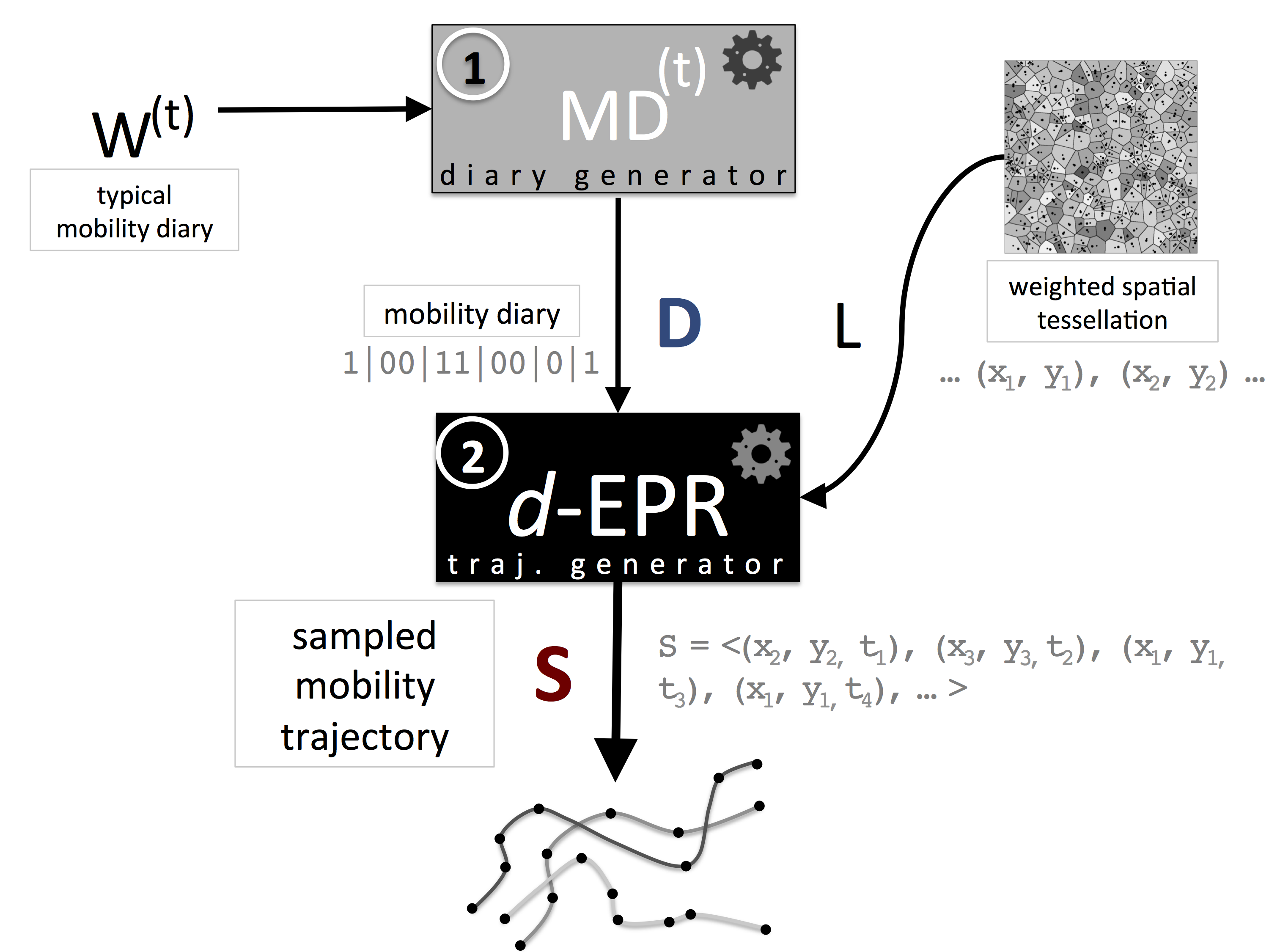
Outline of the DITRAS framework. DITRAS combines two probabilistic models: a diary generator (e.g., \(MD(t)\)) and trajectory generator (e.g., d-EPR). The diary generator produces a mobility diary \(D\). The mobility diary \(D\) is the input of the trajectory generator together with a weighted spatial tessellation of the territory \(L\). From \(D\) and \(L\) the trajectory generator produces a synthetic mobility trajectory \(S\).
- Parameters
diary_generator (MarkovDiaryGenerator) – the diary generator to use for generating the diary.
name (str, optional) – the name of the instantiation of the Ditras model. The default value is “Ditras”.
rho (float, optional) – it corresponds to the parameter \(\rho \in (0, 1]\) in the Action selection mechanism of the DensityEPR model \(P_{new} = \rho S^{-\gamma}\) and controls the agent’s tendency to explore a new location during the next move versus returning to a previously visited location. The default value is \(\rho = 0.6\) [SKWB2010].
gamma (float, optional) – it corresponds to the parameter \(\gamma\) (\(\gamma \geq 0\)) in the Action selection mechanism of the DensityEPR model \(P_{new} = \rho S^{-\gamma}\) and controls the agent’s tendency to explore a new location during the next move versus returning to a previously visited location. The default value is \(\gamma=0.21\) [SKWB2010].
- Variables
diary_generator (MarkovDiaryGenerator) – the diary generator to use for generating the diary [PS2018].
name (str) – the name of the instantiation of the model.
rho (float) – the input parameter \(\rho\).
gamma (float) – the input parameters \(\gamma\).
Examples
>>> import skmob
>>> from skmob.models.epr import Ditras
>>> from skmob.models.markov_diary_generator import MarkovDiaryGenerator
>>> from skmob.preprocessing import filtering, compression, detection, clustering
>>>
>>> # load and preprocess data to train the MarkovDiaryGenerator
>>> url = skmob.utils.constants.GEOLIFE_SAMPLE
>>> df = pd.read_csv(url, sep=',', compression='gzip')
>>> tdf = skmob.TrajDataFrame(df, latitude='lat', longitude='lon', user_id='user', datetime='datetime')
>>> ctdf = compression.compress(tdf)
>>> stdf = detection.stay_locations(ctdf)
>>> cstdf = clustering.cluster(stdf)
>>>
>>> # instantiate and train the MarkovDiaryGenerator
>>> mdg = MarkovDiaryGenerator()
>>> mdg.fit(cstdf, 2, lid='cluster')
>>>
>>> # set start time, end time and tessellation for the simulation
>>> start_time = pd.to_datetime('2019/01/01 08:00:00')
>>> end_time = pd.to_datetime('2019/01/14 08:00:00')
>>> tessellation = gpd.GeoDataFrame.from_file("data/NY_counties_2011.geojson")
>>>
>>> # instantiate the model
>>> ditras = Ditras(mdg)
>>>
>>> # run the model
>>> ditras_tdf = ditras.generate(start_time, end_time, tessellation, relevance_column='population',
                n_agents=3, od_matrix=None, show_progress=True)
>>> print(ditras_tdf.head())
   uid            datetime        lat        lng
0    1 2019-01-01 08:00:00  43.382528 -78.230656
1    1 2019-01-02 03:00:00  43.309133 -77.680414
2    1 2019-01-02 23:00:00  43.382528 -78.230656
3    1 2019-01-03 10:00:00  43.382528 -78.230656
4    1 2019-01-03 21:00:00  43.309133 -77.680414
>>> print(ditras_tdf.parameters)
{'model': {'class': <function Ditras.__init__ at 0x7f0cf0b7e158>, 'generate': {'start_date': Timestamp('2019-01-01 08:00:00'), 'end_date': Timestamp('2019-01-14 08:00:00'), 'gravity_singly': {}, 'n_agents': 3, 'relevance_column': 'population', 'random_state': None, 'show_progress': True}}}
References
- PS2018
Pappalardo, L. & Simini, F. (2018) Data-driven generation of spatio-temporal routines in human mobility. Data Mining and Knowledge Discovery 32, 787-829, https://link.springer.com/article/10.1007/s10618-017-0548-4
See also
DensityEPR,MarkovDiaryGenerator- generate(start_date, end_date, spatial_tessellation, gravity_singly={}, n_agents=1, starting_locations=None, od_matrix=None, relevance_column='relevance', random_state=None, log_file=None, show_progress=False)
Start the simulation of a set of agents at time start_date till time end_date.
- Parameters
start_date (datetime) – the starting date of the simulation, in “YYY/mm/dd HH:MM:SS” format.
end_date (datetime) – the ending date of the simulation, in “YYY/mm/dd HH:MM:SS” format.
spatial_tessellation (geopandas GeoDataFrame) – the spatial tessellation, i.e., a division of the territory in locations.
gravity_singly ({} or Gravity, optional) – the (singly constrained) gravity model to use when generating the probability to move between two locations. The default is “{}”.
n_agents (int, optional) – the number of agents to generate. The default is 1.
starting_locations (list or None, optional) – a list of integers, each identifying the location from which to start the simulation of each agent. Note that, if starting_locations is not None, its length must be equal to the value of n_agents, i.e., you must specify one starting location per agent. The default is None.
od_matrix (numpy array or None, optional) – the origin destination matrix to use for deciding the movements of the agent (element [i,j] is the probability of one trip from location with tessellation index i to j, normalized by origin location). If None, it is computed “on the fly” during the simulation. The default is None.
relevance_column (str, optional) – the name of the column in spatial_tessellation to use as relevance variable. The default is “relevance”.
random_state (int or None, optional) – if int, it is the seed used by the random number generator; if None, the random number generator is the RandomState instance used by np.random and random.random. The default is None.
log_file (str or None, optional) – the name of the file where to write a log of the execution of the model. The logfile will contain all decisions (returns or explorations) made by the model. The default is None.
show_progress (boolean, optional) – if True, show a progress bar. The default is False.
- Returns
the synthetic trajectories generated by the model
- Return type
- class skmob.models.epr.SpatialEPR(name='Spatial EPR model', rho=0.6, gamma=0.21, beta=0.8, tau=17, min_wait_time_minutes=20)
Spatial-EPR model.
The s-EPR model of individual human mobility consists of the following mechanisms [PSRPGB2015] [PSR2016] [SKWB2010]:
Waiting time choice. The waiting time \(\Delta t\) between two movements of the agent is chosen randomly from the distribution \(P(\Delta t) \sim \Delta t^{−1 −\beta} \exp(−\Delta t/ \tau)\). Parameters \(\beta\) and \(\tau\) correspond to arguments beta and tau of the constructor, respectively.
Action selection. With probability \(P_{new}=\rho S^{-\gamma}\), where \(S\) is the number of distinct locations previously visited by the agent, the agent visits a new location (Exploration phase), otherwise it returns to a previously visited location (Return phase). Parameters \(\rho\) and \(\gamma\) correspond to arguments rho and gamma of the constructor, respectively.
Exploration phase. If the agent that is currently in location \(i\) explores a new location, then the new location \(j \neq i\) is selected according to the distance from the current location \(p_{ij} = \frac{1}{r_{ij}^2}\), where \(r_{ij}\) is the geographic distance between \(i\) and \(j\). The number of distinct locations visited, \(S\), is increased by 1.
Return phase. If the individual returns to a previously visited location, such a location \(i\) is chosen with probability proportional to the number of time the agent visited \(i\), i.e., \(\Pi_i = f_i\), where \(f_i\) is the visitation frequency of location \(i\).

Starting at time \(t\) from the configuration shown in the left panel, indicating that the user visited previously \(S=4\) locations with frequency \(f_i\) that is proportional to the size of circles drawn at each location, at time \(t + \Delta t\) (with \(Delta t\) drawn from the \(P(\Delta t)\) fat-tailed distribution) the user can either visit a new location at distance \(\Delta r\) from his/her present location, or return to a previously visited location with probability \(P_{ret}=\rho S^{-\gamma}\), where the next location will be chosen with probability \(\Pi_i=f_i\) (preferential return; lower panel). Figure from [SKWB2010].
- Parameters
name (str, optional) – the name of the instantiation of the s-EPR model. The default value is “Spatial EPR model”.
rho (float, optional) – it corresponds to the parameter \(\rho \in (0, 1]\) in the Action selection mechanism \(P_{new} = \rho S^{-\gamma}\) and controls the agent’s tendency to explore a new location during the next move versus returning to a previously visited location. The default value is \(\rho = 0.6\) [SKWB2010].
gamma (float, optional) – it corresponds to the parameter \(\gamma\) (\(\gamma \geq 0\)) in the Action selection mechanism \(P_{new} = \rho S^{-\gamma}\) and controls the agent’s tendency to explore a new location during the next move versus returning to a previously visited location. The default value is \(\gamma=0.21\) [SKWB2010].
beta (float, optional) – it corresponds to the parameter \(\beta\) of the waiting time distribution in the Waiting time choice mechanism. The default value is \(\beta=0.8\) [SKWB2010].
tau (int, optional) – it corresponds to the parameter \(\tau\) of the waiting time distribution in the Waiting time choice mechanism. The default value is \(\tau = 17\), expressed in hours [SKWB2010].
min_wait_time_minutes (int) – the input parameters min_wait_time_minutes
- Variables
name (str) – the name of the instantiation of the model.
rho (float) – the input parameter \(\rho\).
gamma (float) – the input parameters \(\gamma\).
beta (float) – the input parameter \(\beta\).
tau (int) – the input parameter \(\tau\).
min_wait_time_minutes (int) – the input parameters min_wait_time_minutes.
Examples
>>> import skmob
>>> import pandas as pd
>>> import geopandas as gpd
>>> from skmob.models.epr import SpatialEPR
>>> url = >>> url = skmob.utils.constants.NY_COUNTIES_2011
>>> tessellation = gpd.read_file(url)
>>> start_time = pd.to_datetime('2019/01/01 08:00:00')
>>> end_time = pd.to_datetime('2019/01/14 08:00:00')
>>> sepr = SpatialEPR()
>>> tdf = sepr.generate(start_time, end_time, tessellation, n_agents=100, show_progress=True)
>>> print(tdf.head())
   uid                   datetime        lat        lng
0    1 2019-01-01 08:00:00.000000  42.267915 -77.383591
1    1 2019-01-01 13:06:13.973868  42.633510 -77.105324
2    1 2019-01-01 14:17:41.188668  42.452018 -76.473618
3    1 2019-01-01 14:49:30.896248  42.633510 -77.105324
4    1 2019-01-01 15:10:54.133150  43.382528 -78.230656
>>> print(tdf.parameters)
{'model': {'class': <function SpatialEPR.__init__ at 0x7f548a49e048>, 'generate': {'start_date': Timestamp('2019-01-01 08:00:00'), 'end_date': Timestamp('2019-01-14 08:00:00'), 'gravity_singly': {}, 'n_agents': 100, 'relevance_column': None, 'random_state': None, 'show_progress': True}}}
See also
EPR,DensityEPR,Ditras- generate(start_date, end_date, spatial_tessellation, gravity_singly={}, n_agents=1, starting_locations=None, od_matrix=None, random_state=None, log_file=None, show_progress=False)
Start the simulation of a set of agents at time start_date till time end_date.
- Parameters
start_date (datetime) – the starting date of the simulation, in “YYY/mm/dd HH:MM:SS” format.
end_date (datetime) – the ending date of the simulation, in “YYY/mm/dd HH:MM:SS” format.
spatial_tessellation (geopandas GeoDataFrame) – the spatial tessellation, i.e., a division of the territory in locations.
gravity_singly ({} or Gravity, optional) – the gravity model (singly constrained) to use when generating the probability to move between two locations (note, used by DensityEPR). The default is “{}”.
n_agents (int, optional) – the number of agents to generate. The default is 1.
starting_locations (list or None, optional) – a list of integers, each identifying the location from which to start the simulation of each agent. Note that, if starting_locations is not None, its length must be equal to the value of n_agents, i.e., you must specify one starting location per agent. The default is None.
od_matrix (numpy array or None, optional) – the origin destination matrix to use for deciding the movements of the agent (element [i,j] is the probability of one trip from location with tessellation index i to j, normalized by origin location). If None, it is computed “on the fly” during the simulation. The default is None.
random_state (int or None, optional) – if int, it is the seed used by the random number generator; if None, the random number generator is the RandomState instance used by np.random and random.random. The default is None.
log_file (str or None, optional) – the name of the file where to write a log of the execution of the model. The logfile will contain all decisions (returns or explorations) made by the model. The default is None.
show_progress (boolean, optional) – if True, show a progress bar. The default is False.
- Returns
the synthetic trajectories generated by the model
- Return type
Markov Diary Generator
- class skmob.models.markov_diary_generator.MarkovDiaryGenerator(name='Markov diary')
Markov Diary Learner and Generator.
A diary generator \(G\) produces a mobility diary, \(D(t)\), containing the sequence of trips made by an agent during a time period divided in time slots of \(t\) seconds. For example, \(G(3600)\) and \(G(60)\) produce mobility diaries with temporal resolutions of one hour and one minute, respectively [PS2018].
A Mobility Diary Learner (MDL) is a data-driven algorithm to compute a mobility diary \(MD\) from the mobility trajectories of a set of real individuals. We use a Markov model to describe the probability that an individual follows her routine and visits a typical location at the usual time, or she breaks the routine and visits another location. First, MDL translates mobility trajectory data of real individuals into abstract mobility trajectories. Second, it uses the obtained abstract trajectory data to compute the transition probabilities of the Markov model \(MD(t)\) [PS2018].
- Parameters
name (str, optional) – name of the instantiation of the class. The default is “Markov diary”.
- Variables
name (str) – name of the instantiation of the class.
markov_chain (dict) – the trained markov chain.
time_slot_length (str) – length of the time slot (1h).
Examples
>>> import skmob
>>> import pandas as pd
>>> import geopandas as gpd
>>> from skmob.models.epr import Ditras
>>> from skmob.models.markov_diary_generator import MarkovDiaryGenerator
>>> from skmob.preprocessing import filtering, compression, detection, clustering
>>> url = skmob.utils.constants.GEOLIFE_SAMPLE
>>>
>>> df = pd.read_csv(url, sep=',', compression='gzip')
>>> tdf = skmob.TrajDataFrame(df, latitude='lat', longitude='lon', user_id='user', datetime='datetime')
>>>
>>> ctdf = compression.compress(tdf)
>>> stdf = detection.stops(ctdf)
>>> cstdf = clustering.cluster(stdf)
>>>
>>> mdg = MarkovDiaryGenerator()
>>> mdg.fit(cstdf, 2, lid='cluster')
>>>
>>> start_time = pd.to_datetime('2019/01/01 08:00:00')
>>> diary = mdg.generate(100, start_time)
>>> print(diary)
             datetime  abstract_location
0 2019-01-01 08:00:00                  0
1 2019-01-02 19:00:00                  1
2 2019-01-02 20:00:00                  0
3 2019-01-03 17:00:00                  1
4 2019-01-03 18:00:00                  2
5 2019-01-04 08:00:00                  0
6 2019-01-05 03:00:00                  1
References
- PS2018
Pappalardo, L. & Simini, F. (2018) Data-driven generation of spatio-temporal routines in human mobility. Data Mining and Knowledge Discovery 32, 787-829, https://link.springer.com/article/10.1007/s10618-017-0548-4
See also
Ditras- fit(traj, n_individuals, lid='location')
Train the markov mobility diary from real trajectories.
- Parameters
traj (TrajDataFrame) – the trajectories of the individuals.
n_individuals (int) – the number of individuals in the TrajDataFrame to consider.
lid (string, optional) – the name of the column containing the identifier of the location. The default is “location”.
- generate(diary_length, start_date, random_state=None)
Start the generation of the mobility diary.
- Parameters
diary_length (int) – the length of the diary in hours.
start_date (datetime) – the starting date of the generation.
- Returns
the generated mobility diary.
- Return type
pandas DataFrame
Gravity
- class skmob.models.gravity.Gravity(deterrence_func_type='power_law', deterrence_func_args=[-2.0], origin_exp=1.0, destination_exp=1.0, gravity_type='singly constrained', name='Gravity model')
Gravity model.
The Gravity model of human migration. In its original formulation, the probability \(T_{ij}\) of moving from a location \(i\) to location \(j\) is defined as [Z1946]:
\[T_{ij} \propto \frac{P_i P_j}{r_{ij}}\]where \(P_i\) and \(P_j\) are the population of location \(i\) and \(j\) and \(r_{ij}\) is the distance between \(i\) and \(j\). The basic assumptions of this model are that the number of trips leaving location \(i\) is proportional to its population \(P_i\), the attractivity of location \(j\) is also proportional to \(P_j\), and finally, that there is a cost effect in terms of distance traveled. These ideas can be generalized assuming a relation of the type [BBGJLLMRST2018]:
\[T_{ij} = K m_i m_j f(r_{ij})\]where \(K\) is a constant, the masses \(m_i\) and \(m_j\) relate to the number of trips leaving location \(i\) or the ones attracted by location \(j\), and \(f(r_{ij})\), called deterrence function, is a decreasing function of distance. The deterrence function \(f(r_{ij})\) is commonly modeled with a powerlaw or an exponential form.
Constrained gravity models. Some of the limitations of the gravity model can be resolved via constrained versions. For example, one may hold the number of people originating from a location \(i\) to be a known quantity \(O_i\), and the gravity model is then used to estimate the destination, constituting a so-called singly constrained gravity model of the form:
\[T_{ij} = K_i O_i m_j f(r_{ij}) = O_i \frac{m_i f(r_{ij})}{\sum_k m_k f(r_{ik})}.\]In this formulation, the proportionality constants \(K_i\) depend on the location of the origin and its distance to the other places considered. We can fix also the total number of travelers arriving at a destination \(j\) as \(D_j = \sum_i T_{ij}\), leading to a doubly-constrained gravity model. For each origin-destination pair, the flow is calculated as:
\[T_{ij} = K_i O_i L_j D_j f(r_{ij})\]where there are now two flavors of proportionality constants
\[K_i = \frac{1}{\sum_j L_j D_j f(r_{ij})}, L_j = \frac{1}{\sum_i K_i O_i f(r_{ij})}.\]- Parameters
deterrence_func_type (str, optional) – the deterrence function to use. The possible deterrence function are “power_law” and “exponential”. The default is “power_law”.
deterrence_func_args (list, optional) – the arguments of the deterrence function. The default is [-2.0].
origin_exp (float, optional) – the exponent of the origin’s relevance (only relevant to globally-constrained model). The default is 1.0.
destination_exp (float, optional) – the explonent of the destination’s relevance. The default is 1.0.
gravity_type (str, optional) – the type of gravity model. Possible values are “singly constrained” and “globally constrained”. The default is “singly constrained”.
name (str, optional) – the name of the instantiation of the Gravity model. The default is “Gravity model”.
- Variables
deterrence_func_type (str) – the deterrence function to use. The possible deterrence function are “power_law” and “exponential”.
deterrence_func_args (list) – the arguments of the deterrence function.
origin_exp (float) – the exponent of the origin’s relevance (only relevant to globally-constrained model).
destination_exp (float) – the explonent of the destination’s relevance.
gravity_type (str) – the type of gravity model. Possible values are “singly constrained” and “globally constrained”.
name (str) – the name of the instantiation of the Gravity model.
Examples
>>> import skmob
>>> from skmob.utils import utils, constants
>>> import pandas as pd
>>> import geopandas as gpd
>>> import numpy as np
>>> from skmob.models import Gravity
>>> # load a spatial tessellation
>>> url_tess = skmob.utils.constants.NY_COUNTIES_2011
>>> tessellation = gpd.read_file(url_tess).rename(columns={'tile_id': 'tile_ID'})
>>> print(tessellation.head())
  tile_ID  population                                           geometry
0   36019       81716  POLYGON ((-74.006668 44.886017, -74.027389 44....
1   36101       99145  POLYGON ((-77.099754 42.274215, -77.0996569999...
2   36107       50872  POLYGON ((-76.25014899999999 42.296676, -76.24...
3   36059     1346176  POLYGON ((-73.707662 40.727831, -73.700272 40....
4   36011       79693  POLYGON ((-76.279067 42.785866, -76.2753479999...
>>> # load real flows into a FlowDataFrame
>>> fdf = skmob.FlowDataFrame.from_file(skmob.utils.constants.NY_FLOWS_2011,
                                        tessellation=tessellation,
                                        tile_id='tile_ID',
                                        sep=",")
>>> print(fdf.head())
     flow origin destination
0  121606  36001       36001
1       5  36001       36005
2      29  36001       36007
3      11  36001       36017
4      30  36001       36019
>>> # compute the total outflows from each location of the tessellation (excluding self loops)
>>> tot_outflows = fdf[fdf['origin'] != fdf['destination']].groupby(by='origin', axis=0)[['flow']].sum().fillna(0)
>>> tessellation = tessellation.merge(tot_outflows, left_on='tile_ID', right_on='origin').rename(columns={'flow': constants.TOT_OUTFLOW})
>>> print(tessellation.head())
  tile_id  population                                           geometry      0   36019       81716  POLYGON ((-74.006668 44.886017, -74.027389 44....
1   36101       99145  POLYGON ((-77.099754 42.274215, -77.0996569999...
2   36107       50872  POLYGON ((-76.25014899999999 42.296676, -76.24...
3   36059     1346176  POLYGON ((-73.707662 40.727831, -73.700272 40....
4   36011       79693  POLYGON ((-76.279067 42.785866, -76.2753479999...
   tot_outflow
0        29981
1         5319
2       295916
3         8665
4         8871
>>> # instantiate a singly constrained Gravity model
>>> gravity_singly = Gravity(gravity_type='singly constrained')
>>> print(gravity_singly)
Gravity(name="Gravity model", deterrence_func_type="power_law", deterrence_func_args=[-2.0], origin_exp=1.0, destination_exp=1.0, gravity_type="singly constrained")
>>> np.random.seed(0)
>>> synth_fdf = gravity_singly.generate(tessellation,
                                   tile_id_column='tile_ID',
                                   tot_outflows_column='tot_outflow',
                                   relevance_column= 'population',
                                   out_format='flows')
>>> print(synth_fdf.head())
  origin destination  flow
0  36019       36101   101
1  36019       36107    66
2  36019       36059  1041
3  36019       36011   151
4  36019       36123    33
>>> # fit the parameters of the Gravity model from real fluxes
>>> gravity_singly_fitted = Gravity(gravity_type='singly constrained')
>>> print(gravity_singly_fitted)
Gravity(name="Gravity model", deterrence_func_type="power_law", deterrence_func_args=[-2.0], origin_exp=1.0, destination_exp=1.0, gravity_type="singly constrained")
>>> gravity_singly_fitted.fit(fdf, relevance_column='population')
>>> print(gravity_singly_fitted)
Gravity(name="Gravity model", deterrence_func_type="power_law", deterrence_func_args=[-1.9947152031914186], origin_exp=1.0, destination_exp=0.6471759552223144, gravity_type="singly constrained")
>>> np.random.seed(0)
>>> synth_fdf_fitted = gravity_singly_fitted.generate(tessellation,
                                                        tile_id_column='tile_ID',
                                                        tot_outflows_column='tot_outflow',
                                                        relevance_column= 'population',
                                                        out_format='flows')
>>> print(synth_fdf_fitted.head())
  origin destination  flow
0  36019       36101   102
1  36019       36107    66
2  36019       36059  1044
3  36019       36011   152
4  36019       36123    33
References
- Z1946
Zipf, G. K. (1946) The P 1 P 2/D hypothesis: on the intercity movement of persons. American sociological review 11(6), 677-686, https://www.jstor.org/stable/2087063?seq=1#metadata_info_tab_contents
- W1971
Wilson, A. G. (1971) A family of spatial interaction models, and associated developments. Environment and Planning A 3(1), 1-32, https://econpapers.repec.org/article/pioenvira/v_3a3_3ay_3a1971_3ai_3a1_3ap_3a1-32.htm
- BBGJLLMRST2018
Barbosa, H., Barthelemy, M., Ghoshal, G., James, C. R., Lenormand, M., Louail, T., Menezes, R., Ramasco, J. J. , Simini, F. & Tomasini, M. (2018) Human mobility: Models and applications. Physics Reports 734, 1-74, https://www.sciencedirect.com/science/article/abs/pii/S037015731830022X
See also
Radiation- fit(flow_df, relevance_column='relevance')
Fit the parameters of the Gravity model to the flows provided in input, using a Generalized Linear Model (GLM) with a Poisson regression [FM1982].
- Parameters
flow_df (FlowDataFrame) – the real flows on the spatial tessellation.
relevance_column (str, optional) – the column in the spatial tessellation with the relevance of the location. The default is constants.RELEVANCE.
References
- FM1982
Flowerdew, R. & Murray, A. (1982) A method of fitting the gravity model based on the Poisson distribution. Journal of regional science 22(2), 191-202, https://onlinelibrary.wiley.com/doi/abs/10.1111/j.1467-9787.1982.tb00744.x
- generate(spatial_tessellation, tile_id_column='tile_ID', tot_outflows_column='tot_outflow', relevance_column='relevance', out_format='flows')
Start the simulation of the Gravity model.
- Parameters
spatial_tessellation (GeoDataFrame) – the spatial tessellation on which to run the simulation.
tile_id_column (str, optional) – the column in spatial_tessellation of the location identifier. The default is constants.TILE_ID.
tot_outflows_column (str, optional) – the column in spatial_tessellation with the outflow of the location. The default is constants.TOT_OUTFLOW.
relevance_column (str, optional) – the column in spatial_tessellation with the relevance of the location. The default is constants.RELEVANCE.
out_format (str, optional) – the format of the generated flows. Possible values are “flows” (average flow between two locations), “flows_sample” (random sample of flows), and “probabilities” (probability of a unit flow between two locations). The default is “flows”.
- Returns
the flows generated by the Gravity model.
- Return type
Radiation
- class skmob.models.radiation.Radiation(name='Radiation model')
Radiation model.
The radiation model for human migration. The radiation model assumes that the choice of a traveler’s destination consists of two steps. First, each opportunity in every location is assigned a fitness represented by a number \(z\), chosen from some distribution \(P(z)\) whose value represents the quality of the opportunity for the traveler. Second, the traveler ranks all opportunities according to their distances from the origin location and chooses the closest opportunity with a fitness higher than the traveler’s fitness threshold, which is another random number extracted from the fitness distribution \(P(z)\). As a result, the average number of travelers from location \(i\) to location \(j\) takes the form [SGMB2012]:
\[T_{ij} = O_i \frac{1}{1 - \frac{m_i}{M}}\frac{m_i m_j}{(m_i + s_{ij})(m_i + m_j + s_{ij})}.\]The destination of the \(O_i\) trips originating in \(i\) is sampled from a distribution of probabilities that a trip originating in \(i\) ends in location \(j\). This probability depends on the number of opportunities at the origin \(m_i\), at the destination \(m_j\) and the number of opportunities \(s_{ij}\) in a circle of radius \(r_{ij}\) centered in \(i\) (excluding the source and destination). This conditional probability needs to be normalized so that the probability that a trip originating in the region of interest ends in this region is equal to 1. In case of a finite system it is possible to show that this is equal to \(1 - \frac{m_i}{M}\) where \(M=\sum_i m_i\) is the total number of opportunities. In the original version of the radiation model, the number of opportunities is approximated by the population, but the total inflows \(D_j\) to each destination can also be used.
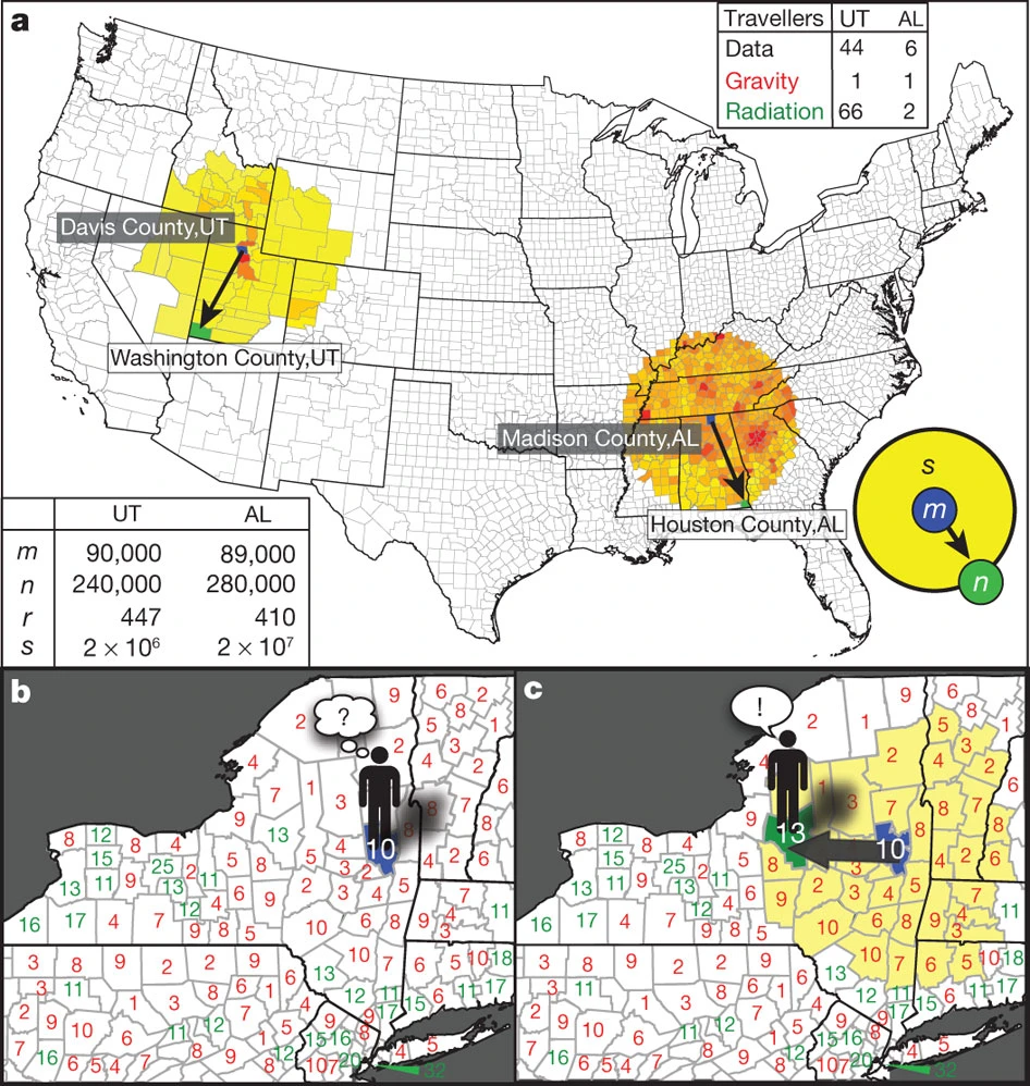
(a) To demonstrate the limitations of the gravity law we highlight two pairs of counties, one in Utah (UT) and the other in Alabama (AL), with similar origin (\(m\), blue) and destination (\(n\), green) populations and comparable distance \(r\) between them (see bottom left table). The US census 2000 reports a flux that is an order of magnitude greater between the Utah counties, a difference correctly captured by the radiation model (b, c). (b) The definition of the radiation model: an individual (for example, living in Saratoga County, New York) applies for jobs in all counties and collects potential employment offers. The number of job opportunities in each county (\(j\)) is \(n_j / n_{jobs}\), chosen to be proportional to the resident population \(n_j\). Each offer’s attractiveness (benefit) is represented by a random variable with distribution \(P(z)\), the numbers placed in each county representing the best offer among the \(n_j / n_{jobs}\) trials in that area. Each county is marked in green (red) if its best offer is better (lower) than the best offer in the home county (here \(z = 10\)). (c) An individual accepts the closest job that offers better benefits than his home county. In the shown configuration the individual will commute to Oneida County, New York, the closest county whose benefit \(z = 13\) exceeds the home county benefit \(z = 10\). This process is repeated for each potential commuter, choosing new benefit variables \(z\) in each case. Figure from [SGMB2012].
- Parameters
name (str, optional) – the name of the instantiation of the radiation model. The default is ‘Radiation model’.
- Variables
name (str) – the name of the instantiation of the model.
Examples
>>> import skmob
>>> from skmob.utils import utils, constants
>>> import pandas as pd
>>> import geopandas as gpd
>>> import numpy as np
>>> from skmob.models import Radiation
>>> # load a spatial tessellation
>>> url_tess = skmob.utils.constants.NY_COUNTIES_2011
>>> tessellation = gpd.read_file(url_tess).rename(columns={'tile_id': 'tile_ID'})
>>> print(tessellation.head())
  tile_ID  population                                           geometry
0   36019       81716  POLYGON ((-74.006668 44.886017, -74.027389 44....
1   36101       99145  POLYGON ((-77.099754 42.274215, -77.0996569999...
2   36107       50872  POLYGON ((-76.25014899999999 42.296676, -76.24...
3   36059     1346176  POLYGON ((-73.707662 40.727831, -73.700272 40....
4   36011       79693  POLYGON ((-76.279067 42.785866, -76.2753479999...
>>> # load real flows into a FlowDataFrame
>>> fdf = skmob.FlowDataFrame.from_file(skmob.utils.constants.NY_FLOWS_2011,
                                        tessellation=tessellation,
                                        tile_id='tile_ID',
                                        sep=",")
>>> print(fdf.head())
     flow origin destination
0  121606  36001       36001
1       5  36001       36005
2      29  36001       36007
3      11  36001       36017
4      30  36001       36019
>>> # compute the total outflows from each location of the tessellation (excluding self loops)
>>> tot_outflows = fdf[fdf['origin'] != fdf['destination']].groupby(by='origin', axis=0)[['flow']].sum().fillna(0)
>>> tessellation = tessellation.merge(tot_outflows, left_on='tile_ID', right_on='origin').rename(columns={'flow': constants.TOT_OUTFLOW})
>>> print(tessellation.head())
  tile_id  population                                           geometry      0   36019       81716  POLYGON ((-74.006668 44.886017, -74.027389 44....
1   36101       99145  POLYGON ((-77.099754 42.274215, -77.0996569999...
2   36107       50872  POLYGON ((-76.25014899999999 42.296676, -76.24...
3   36059     1346176  POLYGON ((-73.707662 40.727831, -73.700272 40....
4   36011       79693  POLYGON ((-76.279067 42.785866, -76.2753479999...
   tot_outflow
0        29981
1         5319
2       295916
3         8665
4         8871
>>> np.random.seed(0)
>>> radiation = Radiation()
>>> rad_flows = radiation.generate(tessellation, tile_id_column='tile_ID',  tot_outflows_column='tot_outflow', relevance_column='population', out_format='flows_sample')
>>> print(rad_flows.head())
  origin destination   flow
0  36019       36033  11648
1  36019       36031   4232
2  36019       36089   5598
3  36019       36113   1596
4  36019       36041    117
References
- SGMB2012(1,2)
Simini, F., Gonzàlez, M. C., Maritan, A. & Barabasi, A.-L. (2012) A universal model for mobility and migration patterns. Nature 484(7392), 96-100, https://www.nature.com/articles/nature10856
- MSJB2013
Masucci, A. P., Serras, J., Johansson, A., & Batty, M. (2013). Gravity versus radiation models: On the importance of scale and heterogeneity in commuting flows. Physical Review E, 88(2), 022812.
- generate(spatial_tessellation, tile_id_column='tile_ID', tot_outflows_column='tot_outflow', relevance_column='relevance', out_format='flows')
Start the simulation of the Radiation model.
- Parameters
spatial_tessellation (GeoDataFrame) – the spatial tessellation on which to perform the simulation.
tile_id_column (str, optional) – the column in spatial_tessellation of the location identifier. The default is constants.TILE_ID.
tot_outflows_column (str, optional) – the column in spatial_tessellation with the outflow of the location. The default is constants.TOT_OUTFLOW.
relevance_column (str, optional) – the column in spatial_tessellation with the relevance of the location. The default is constants.RELEVANCE.
out_format (str, optional) – the format of the generated flows. Possible values are: “flows” (average flow between two locations), “flows_sample” (random sample of flows), and “probabilities” (probability of a unit flow between two locations). The default is “flows”.
- Returns
the fluxes generated by the Radiation model.
- Return type
GeoSim
- class skmob.models.geosim.GeoSim(name='GeoSim', rho=0.6, gamma=0.21, alpha=0.2, beta=0.8, tau=17, min_wait_time_hours=1)
GeoSim model.
The GeoSim model of individual human mobility consists of the following mechanisms [THSG2015]:
Waiting time choice. The waiting time \(\Delta t\) between two movements of the agent is chosen randomly from the distribution \(P(\Delta t) \sim \Delta t^{−1 −\beta} \exp(−\Delta t/ \tau)\). Parameters \(\beta\) and \(\tau\) correspond to arguments beta and tau of the constructor, respectively.
Action selection. With probability \(P_{exp}=\rho S^{-\gamma}\), where \(S\) is the number of distinct locations previously visited by the agent, the agent visits a new location (Exploration), otherwise with a complementary probability \(P_{ret}=1-P{exp}\) it returns to a previously visited location (Return). At that point, the agent determines whether or not the location’s choice will be affected by the other agents; with a probability \(\alpha\), the agent’s social contacts influence its movement (Social). With a complementary probability of \(1-\alpha\), the agent’s choice is not influenced by the other agents (Individual).
Parameters \(\rho\), \(\gamma\), and \(\alpha=\) correspond to arguments rho, gamma, and alpha of the constructor, respectively.
After the selection of the spatial mechanism (Exploration or Return) and the social mechanism (Individual or Social) decides which location will be the destination of its next displacement during the Location selection phase. For an agent \(a\), we denote the sets containing the indices of the locations \(a\) can explore or return, as \(exp_{a}\) and \(ret_{a}\), respectively.
Individual Exploration. If the agent \(a\) is currently in location \(i\), and explores a new location without the influence of its social contacts, then the new location \(j \neq i\) is an unvisited location for the agent (\(i \in exp_{a}\)) and it is selected with probability proportional to \(\frac{1}{|exp_{a}|}\). The number of distinct locations visited, \(S\), is increased by 1.
Social Exploration. If the agent \(a\) is currently in location \(i\), and explores a new location with the influence of a social contact, it first selects a social contact \(c\) with probability \(p(c) \propto mob_{sim}(a,c)\) [THSG2015]. At this point, the agent \(a\) explores an unvisited location for agent \(a\) that was visited by agent \(c\), i.e., the location \(j \neq i\) is selected from set \(A = exp_a \cap ret_c\); the probability \(p(j)\) for a location \(j \in A\), to be selected is proportional to \(\Pi_j = f_j\), where \(f_j\) is the visitation frequency of location \(j\) for the agent \(c\). The number of distinct locations visited, \(S\), is increased by 1.
Individual Return. If the agent \(a\), currently at location \(i\), returns to a previously visited location \(j \in ret_a\), it is chosen with probability proportional to the number of time the agent visited \(j\), i.e., \(\Pi_j = f_j\), where \(f_j\) is the visitation frequency of location \(j\).
Social Return. If the agent \(a\) is currently in location \(i\), and returns to a previously visited location with the influence of a social contact, it first selects a social contact \(c\) with probability \(p(c) \propto mob_{sim}(a,c)\) [THSG2015]. At this point, the agent \(a\) returns to a previously visited location for agent \(a\) that was visited by agent \(c\) too, i.e., the location \(j \neq i\) is selected from set \(A = ret_a \cap ret_c\); the probability \(p(j)\) for a location \(j \in A\), to be selected is proportional to \(\Pi_j = f_j\), where \(f_j\) is the visitation frequency of location \(j\) for the agent \(c\).
- Parameters
name (str, optional) – the name of the instantiation of the GeoSim model. The default value is “GeoSim”.
rho (float, optional) – it corresponds to the parameter \(\rho \in (0, 1]\) in the Action selection mechanism \(P_{exp} = \rho S^{-\gamma}\) and controls the agent’s tendency to explore a new location during the next move versus returning to a previously visited location. The default value is \(\rho = 0.6\) [SKWB2010].
gamma (float, optional) – it corresponds to the parameter \(\gamma\) (\(\gamma \geq 0\)) in the Action selection mechanism \(P_{exp} = \rho S^{-\gamma}\) and controls the agent’s tendency to explore a new location during the next move versus returning to a previously visited location. The default value is \(\gamma=0.21\) [SKWB2010].
alpha (float, optional) – it corresponds to the parameter alpha in the Action selection mechanism and controls the influence of the social contacts for an agent during its location selection phase. The default value is \(\alpha=0.2\) [THSG2015].
beta (float, optional) – it corresponds to the parameter \(\beta\) of the waiting time distribution in the Waiting time choice mechanism. The default value is \(\beta=0.8\) [SKWB2010].
tau (int, optional) – it corresponds to the parameter \(\tau\) of the waiting time distribution in the Waiting time choice mechanism. The default value is \(\tau = 17\), expressed in hours [SKWB2010].
min_wait_time_minutes (int) – minimum waiting time between two movements, in hours.
- Variables
name (str) – the name of the instantiation of the model.
rho (float) – the input parameter \(\rho\).
gamma (float) – the input parameters \(\gamma\).
alpha (float) – the input parameter \(\alpha\).
beta (float) – the input parameter \(\beta\).
tau (int) – the input parameter \(\tau\).
min_wait_time_minutes (int) – the input parameters min_wait_time_minutes.
References
- PSRPGB2015
Pappalardo, L., Simini, F. Rinzivillo, S., Pedreschi, D. Giannotti, F. & Barabasi, A. L. (2015) Returners and Explorers dichotomy in human mobility. Nature Communications 6, https://www.nature.com/articles/ncomms9166
- PSR2016
Pappalardo, L., Simini, F. Rinzivillo, S. (2016) Human Mobility Modelling: exploration and preferential return meet the gravity model. Procedia Computer Science 83, https://www.sciencedirect.com/science/article/pii/S1877050916302216
- SKWB2010
Song, C., Koren, T., Wang, P. & Barabasi, A.L. (2010) Modelling the scaling properties of human mobility. Nature Physics 6, 818-823, https://www.nature.com/articles/nphys1760
- THSG2015
Toole, Jameson & Herrera-Yague, Carlos & Schneider, Christian & Gonzalez, Marta C.. (2015). Coupling Human Mobility and Social Ties. Journal of the Royal Society, Interface / the Royal Society. 12. 10.1098/rsif.2014.1128.
See also
EPR,SpatialEPR,Ditras- action_correction(agent, choice)
The implementation of the action-correction phase, executed by an agent if the location selection phase does not allow movements in any location
- cosine_similarity(x, y)
Cosine Similarity (x,y) = <x,y>/(||x||*||y||)
- generate(start_date, end_date, spatial_tessellation, social_graph='random', n_agents=500, dt_update_mobSim=168, indipendency_window=0.5, random_state=None, log_file=None, verbose=0, show_progress=False)
Start the simulation of a set of agents at time start_date till time end_date.
- Parameters
start_date (datetime) – the starting date of the simulation, in “YYY/mm/dd HH:MM:SS” format.
end_date (datetime) – the ending date of the simulation, in “YYY/mm/dd HH:MM:SS” format.
spatial_tessellation (pandas DataFrame or geopandas GeoDataFrame) – the spatial tessellation, i.e., a division of the territory in locations.
social_graph (“random” or an edge list) – the social graph describing the sociality of the agents. The default is “random”.
n_agents (int, optional) – the number of agents to generate. If social_graph is “random”, n_agents are initialized and connected, otherwise the number of agents is inferred from the edge list. The default is 500.
random_state (int or None, optional) – if int, it is the seed used by the random number generator; if None, the random number generator is the RandomState instance used by np.random and random.random. The default is None.
dt_update_mobSim (float, optional) – the time interval (in hours) that specifies how often to update the weights of the social graph. The default is 24*7=168 (one week).
indipendency_window (float, optional) – the time window (in hours) that must elapse before an agent’s movements can affect the movements of other agents in the simulation. The default is 0.5.
log_file (str or None, optional) – the name of the file where to write a log of the execution of the model. The logfile will contain all decisions made by the model. The default is None.
verbose (int, optional) – the verbosity level of the model relative to the standard output. If verbose is equal to 2 the initialization info and the decisions made by the model are printed, if verbose is equal to 1 only the initialization info are reported. The default is 0.
show_progress (boolean, optional) – if True, show a progress bar. The default is False.
- Returns
the synthetic trajectories generated by the model
- Return type
- make_individual_exploration_action(agent)
The agent A selects uniformly at random an UNVISITED location (i.e., in exp(A))
- make_individual_return_action(agent)
The agent A makes a preferential choice selecting a VISITED location (i.e., in ret(A)) with probability proportional to the number of visits to that location.
- make_social_action(agent, mode)
The agent A makes a social choice in the following way:
1. The agent A selects a social contact C with probability proportional to the mobility similarity between them
2. The candidate location to visit or explore is selected from the set composed of the locations visited by C (ret(C)), that are feasible according to A’s action:
exploration: exp(A) intersect ret(C)
return: ret(A) intersect ret(C)
3. select one of the feasible locations (if any) with a probability proportional to C’s visitation frequency
STS-EPR
- class skmob.models.sts_epr.STS_epr(name='STS-EPR', rho=0.6, gamma=0.21, alpha=0.2)
STS-EPR model.
The STS-EPR (Spatial, Temporal and Social EPR model) model of individual human mobility consists of the following mechanisms [CRP2020]:
Action selection. With probability \(P_{exp}=\rho S^{-\gamma}\), where \(S\) is the number of distinct locations previously visited by the agent, the agent visits a new location (Exploration), otherwise with a complementary probability \(P_{ret}=1-P{exp}\) it returns to a previously visited location (Return). At that point, the agent determines whether or not the location’s choice will be affected by the other agents; with a probability \(\alpha\), the agent’s social contacts influence its movement (Social). With a complementary probability of \(1-\alpha\), the agent’s choice is not influenced by the other agents (Individual).
Parameters \(\rho\), \(\gamma\), and \(\alpha=\) correspond to arguments rho, gamma, and alpha of the constructor, respectively.
After the selection of the spatial mechanism (Exploration or Return) and the social mechanism (Individual or Social) decides which location will be the destination of its next displacement during the Location selection phase. For an agent \(a\), we denote the sets containing the indices of the locations \(a\) can explore or return, as \(exp_{a}\) and \(ret_{a}\), respectively.
Individual Exploration. If the agent \(a\) is currently in location \(i\), and explores a new location without the influence of its social contacts, then the new location \(j \neq i\) is an unvisited location for the agent (\(i \in exp_{a}\)) and it is selected according to the gravity model with probability proportional to \(p_{ij} = \frac{r_i r_j}{dist_{ij}^2}\), where \(r_{i (j)}\) is the location’s relevance, that is, the probability of a population to visit location \(i(j)\), \(dist_{ij}\) is the geographic distance between \(i\) and \(j\),
The number of distinct locations visited, \(S\), is increased by 1.
Social Exploration. If the agent \(a\) is currently in location \(i\), and explores a new location with the influence of a social contact, it first selects a social contact \(c\) with probability \(p(c) \propto mob_{sim}(a,c)\) [THSG2015]. At this point, the agent \(a\) explores an unvisited location for agent \(a\) that was visited by agent \(c\), i.e., the location \(j \neq i\) is selected from set \(A = exp_a \cap ret_c\); the probability \(p(j)\) for a location \(j \in A\), to be selected is proportional to \(\Pi_j = f_j\), where \(f_j\) is the visitation frequency of location \(j\) for the agent \(c\). The number of distinct locations visited, \(S\), is increased by 1.
Individual Return. If the agent \(a\), currently at location \(i\), returns to a previously visited location \(j \in ret_a\), it is chosen with probability proportional to the number of time the agent visited \(j\), i.e., \(\Pi_j = f_j\), where \(f_j\) is the visitation frequency of location \(j\).
Social Return. If the agent \(a\) is currently in location \(i\), and returns to a previously visited location with the influence of a social contact, it first selects a social contact \(c\) with probability \(p(c) \propto mob_{sim}(a,c)\) [THSG2015]. At this point, the agent \(a\) returns to a previously visited location for agent \(a\) that was visited by agent \(c\) too, i.e., the location \(j \neq i\) is selected from set \(A = ret_a \cap ret_c\); the probability \(p(j)\) for a location \(j \in A\), to be selected is proportional to \(\Pi_j = f_j\), where \(f_j\) is the visitation frequency of location \(j\) for the agent \(c\).
- Parameters
name (str, optional) – the name of the instantiation of the STS-EPR model. The default value is “STS-EPR”.
rho (float, optional) – it corresponds to the parameter \(\rho \in (0, 1]\) in the Action selection mechanism \(P_{exp} = \rho S^{-\gamma}\) and controls the agent’s tendency to explore a new location during the next move versus returning to a previously visited location. The default value is \(\rho = 0.6\) [SKWB2010].
gamma (float, optional) – it corresponds to the parameter \(\gamma\) (\(\gamma \geq 0\)) in the Action selection mechanism \(P_{exp} = \rho S^{-\gamma}\) and controls the agent’s tendency to explore a new location during the next move versus returning to a previously visited location. The default value is \(\gamma=0.21\) [SKWB2010].
alpha (float, optional) – it corresponds to the parameter alpha in the Action selection mechanism and controls the influence of the social contacts for an agent during its location selection phase. The default value is \(\alpha=0.2\) [THSG2015].
- Variables
name (str) – the name of the instantiation of the model.
rho (float) – the input parameter \(\rho\).
gamma (float) – the input parameters \(\gamma\).
alpha (float) – the input parameter \(\alpha\).
References
- PSRPGB2015
Pappalardo, L., Simini, F. Rinzivillo, S., Pedreschi, D. Giannotti, F. & Barabasi, A. L. (2015) Returners and Explorers dichotomy in human mobility. Nature Communications 6, https://www.nature.com/articles/ncomms9166
- PSR2016
Pappalardo, L., Simini, F. Rinzivillo, S. (2016) Human Mobility Modelling: exploration and preferential return meet the gravity model. Procedia Computer Science 83, https://www.sciencedirect.com/science/article/pii/S1877050916302216
- SKWB2010
Song, C., Koren, T., Wang, P. & Barabasi, A.L. (2010) Modelling the scaling properties of human mobility. Nature Physics 6, 818-823, https://www.nature.com/articles/nphys1760
- THSG2015
Toole, Jameson & Herrera-Yague, Carlos & Schneider, Christian & Gonzalez, Marta C.. (2015). Coupling Human Mobility and Social Ties. Journal of the Royal Society, Interface / the Royal Society. 12. 10.1098/rsif.2014.1128.
- CRP2020
Cornacchia, Giuliano & Rossetti, Giulio & Pappalardo, Luca. (2020). Modelling Human Mobility considering Spatial,Temporal and Social Dimensions.
- PS2018
Pappalardo, L. & Simini, F. (2018) Data-driven generation of spatio-temporal routines in human mobility. Data Mining and Knowledge Discovery 32, 787-829, https://link.springer.com/article/10.1007/s10618-017-0548-4
See also
EPR,SpatialEPR,Ditras- action_correction_diary(agent, choice)
The implementation of the action-correction phase, executed by an agent if the location selection phase does not allow movements in any location
- cosine_similarity(x, y)
Cosine Similarity (x,y) = <x,y>/(||x||*||y||)
- generate(start_date, end_date, spatial_tessellation, diary_generator, social_graph='random', n_agents=500, rsl=False, distance_matrix=None, relevance_column=None, min_relevance=0.1, dt_update_mobSim=168, indipendency_window=0.5, random_state=None, log_file=None, verbose=0, show_progress=False)
Start the simulation of a set of agents at time start_date till time end_date.
- Parameters
start_date (datetime) – the starting date of the simulation, in “YYY/mm/dd HH:MM:SS” format.
end_date (datetime) – the ending date of the simulation, in “YYY/mm/dd HH:MM:SS” format.
spatial_tessellation (pandas DataFrame or geopandas GeoDataFrame) – the spatial tessellation, i.e., a division of the territory in locations.
diary_generator (MarkovDiaryGenerator) – the diary generator to use for generating the mobility diary [PS2018].
social_graph (“random” or an edge list) – the social graph describing the sociality of the agents. The default is “random”.
n_agents (int, optional) – the number of agents to generate. If social_graph is “random”, n_agents are initialized and connected, otherwise the number of agents is inferred from the edge list. The default is 500.
rsl (bool, optional) – if Truen the probability \(p(i)\) for an agent of being assigned to a starting physical location \(i\) is proportional to the relevance of location \(i\); otherwise, if False, it is selected uniformly at random. The defailt is False.
distance_matrix (numpy array or None, optional) – the origin destination matrix to use for deciding the movements of the agent. If None, it is computed “on the fly” during the simulation. The default is None.
relevance_column (str, optional) – the name of the column in spatial_tessellation to use as relevance variable. The default is “relevance”.
min_relevance (float, optional) – the value in which to map the null relevance. The default is 0.1.
random_state (int or None, optional) – if int, it is the seed used by the random number generator; if None, the random number generator is the RandomState instance used by np.random and random.random. The default is None.
dt_update_mobSim (float, optional) – the time interval (in hours) that specifies how often to update the weights of the social graph. The default is 24*7=168 (one week).
indipendency_window (float, optional) – the time window (in hours) that must elapse before an agent’s movements can affect the movements of other agents in the simulation. The default is 0.5.
log_file (str or None, optional) – the name of the file where to write a log of the execution of the model. The logfile will contain all decisions made by the model. The default is None.
verbose (int, optional) – the verbosity level of the model relative to the standard output. If verbose is equal to 2 the initialization info and the decisions made by the model are printed, if verbose is equal to 1 only the initialization info are reported. The default is 0.
show_progress (boolean, optional) – if True, show a progress bar. The default is False.
- Returns
the synthetic trajectories generated by the model
- Return type
- make_individual_exploration_action(agent)
The agent A, current at location i selects an UNVISITED location (i.e., in exp(A)) j with probability proportional to (r_i * r_j)/ d_ij^2
- make_individual_return_action(agent)
The agent A makes a preferential choice selecting a VISITED location (i.e., in ret(A)) with probability proportional to the number of visits to that location.
- make_social_action(agent, mode)
The agent A makes a social choice in the following way:
1. The agent A selects a social contact C with probability proportional to the mobility similarity between them
2. The candidate location to visit or explore is selected from the set composed of the locations visited by C (ret(C)), that are feasible according to A’s action:
exploration: exp(A) intersect ret(C)
return: ret(A) intersect ret(C)
3. select one of the feasible locations (if any) with a probability proportional to C’s visitation frequency