Data Structures
scikit-mobility provides two different data structures, both extending the Pandas dataframe: TrajDataframe is designed to deal with trajectories, i.e., data in form of GPS points; FlowDataFrame allows to manage fluxes between places.
TrajDataframe
- class skmob.core.trajectorydataframe.TrajDataFrame(data, latitude='lat', longitude='lng', datetime='datetime', user_id='uid', trajectory_id='tid', timestamp=False, crs={'init': 'epsg:4326'}, parameters={})
TrajDataFrame.
A TrajDataFrame object is a pandas.DataFrame that has three columns latitude, longitude and datetime. TrajDataFrame accepts the following keyword arguments:
- Parameters
data (list or dict or pandas DataFrame) – the data that must be embedded into a TrajDataFrame.
latitude (int or str, optional) – the position or the name of the column in data containing the latitude. The default is constants.LATITUDE.
longitude (int or str, optional) – the position or the name of the column in data containing the longitude. The default is constants.LONGITUDE.
datetime (int or str, optional) – the position or the name of the column in data containing the datetime. The default is constants.DATETIME.
user_id (int or str, optional) – the position or the name of the column in data`containing the user identifier. The default is `constants.UID.
trajectory_id (int or str, optional) – the position or the name of the column in data containing the trajectory identifier. The default is constants.TID.
timestamp (boolean, optional) – it True, the datetime is a timestamp. The default is False.
crs (dict, optional) – the coordinate reference system of the geographic points. The default is {“init”: “epsg:4326”}.
parameters (dict, optional) – parameters to add to the TrajDataFrame. The default is {} (no parameters).
Examples
>>> import skmob
>>> # create a TrajDataFrame from a list
>>> data_list = [[1, 39.984094, 116.319236, '2008-10-23 13:53:05'],
 [1, 39.984198, 116.319322, '2008-10-23 13:53:06'],
 [1, 39.984224, 116.319402, '2008-10-23 13:53:11'],
 [1, 39.984211, 116.319389, '2008-10-23 13:53:16']]
>>> tdf = skmob.TrajDataFrame(data_list, latitude=1, longitude=2, datetime=3)
>>> print(tdf.head())
   0        lat         lng            datetime
0  1  39.984094  116.319236 2008-10-23 13:53:05
1  1  39.984198  116.319322 2008-10-23 13:53:06
2  1  39.984224  116.319402 2008-10-23 13:53:11
3  1  39.984211  116.319389 2008-10-23 13:53:16
>>> print(type(tdf))
<class 'skmob.core.trajectorydataframe.TrajDataFrame'>
>>>
>>> # create a TrajDataFrame from a pandas DataFrame
>>> import pandas as pd
>>> # create a DataFrame from the previous list
>>> data_df = pd.DataFrame(data_list, columns=['user', 'latitude', 'lng', 'hour'])
>>> print(type(data_df))
<class 'pandas.core.frame.DataFrame'>
>>> tdf = skmob.TrajDataFrame(data_df, latitude='latitude', datetime='hour', user_id='user')
>>> print(type(tdf))
<class 'skmob.core.trajectorydataframe.TrajDataFrame'>
>>> print(tdf.head())
   uid        lat         lng            datetime
0    1  39.984094  116.319236 2008-10-23 13:53:05
1    1  39.984198  116.319322 2008-10-23 13:53:06
2    1  39.984224  116.319402 2008-10-23 13:53:11
3    1  39.984211  116.319389 2008-10-23 13:53:16
- classmethod from_file(filename, latitude='lat', longitude='lng', datetime='datetime', user_id='uid', trajectory_id='tid', encoding=None, usecols=None, header='infer', timestamp=False, crs={'init': 'epsg:4326'}, sep=',', parameters=None)
Read a trajectory file and return a TrajDataFrame.
- Parameters
filename (str) – the path to the file
latitude (str, optional) – the name of the column containing the latitude values
longitude (str, optional) – the name of the column containing the longitude values
datetime (str, optional) – the name of the column containing the datetime values
user_id (str, optional) – the name of the column containing the user id values
trajectory_id (str, optional) – the name of the column containing the trajectory id values
encoding (str, optional) – the encoding of the file
usecols (list, optional) – the columns to read
header (int, optional) – the row number of the header
timestamp (bool, optional) – if True, the datetime column contains timestamps
crs (dict, optional) – the coordinate reference system of the TrajDataFrame
sep (str, optional) – the separator of the file
parameters (dict, optional) – the parameters of the TrajDataFrame
- Returns
The loaded TrajDataFrame
- Return type
- mapping(tessellation, remove_na=False)
Assign each point of the TrajDataFrame to the corresponding tile of a spatial tessellation.
- Parameters
tessellation (GeoDataFrame) – the spatial tessellation containing a geometry column with points or polygons.
remove_na (boolean, optional) – if True, remove points that do not have a corresponding tile in the spatial tessellation. The default is False.
- Returns
a TrajDataFrame with an additional column tile_ID indicating the tile identifiers.
- Return type
Examples
>>> import skmob
>>> from skmob.tessellation import tilers
>>> import pandas as pd
>>> from skmob.preprocessing import filtering
>>> # read the trajectory data (GeoLife, Beijing, China)
>>> url = skmob.utils.constants.GEOLIFE_SAMPLE
>>> df = pd.read_csv(url, sep=',', compression='gzip')
>>> tdf = skmob.TrajDataFrame(df, latitude='lat', longitude='lon', user_id='user', datetime='datetime')
>>> print(tdf.head())
         lat         lng            datetime  uid
0  39.984094  116.319236 2008-10-23 05:53:05    1
1  39.984198  116.319322 2008-10-23 05:53:06    1
2  39.984224  116.319402 2008-10-23 05:53:11    1
3  39.984211  116.319389 2008-10-23 05:53:16    1
4  39.984217  116.319422 2008-10-23 05:53:21    1
>>> # build a tessellation over the city
>>> tessellation = tilers.tiler.get("squared", base_shape="Beijing, China", meters=15000)
>>> mtdf = tdf.mapping(tessellation)
>>> print(mtdf.head())
         lat         lng            datetime  uid tile_ID
0  39.984094  116.319236 2008-10-23 05:53:05    1      63
1  39.984198  116.319322 2008-10-23 05:53:06    1      63
2  39.984224  116.319402 2008-10-23 05:53:11    1      63
3  39.984211  116.319389 2008-10-23 05:53:16    1      63
4  39.984217  116.319422 2008-10-23 05:53:21    1      63
- plot_diary(user, start_datetime=None, end_datetime=None, ax=None, legend=False)
Plot a mobility diary of an individual in a TrajDataFrame. It requires a TrajDataFrame with clusters, output of preprocessing.clustering.cluster. The column constants.CLUSTER must be present.
- Parameters
user (str or int) – user identifier whose diary should be plotted.
start_datetime (datetime.datetime, optional) – only stops made after this date will be plotted. If None the datetime of the oldest stop will be selected. The default is None.
end_datetime (datetime.datetime, optional) – only stops made before this date will be plotted. If None the datetime of the newest stop will be selected. The default is None.
ax (matplotlib.axes, optional) – axes where the diary will be plotted. If None a new ax is created. The default is None.
legend (bool, optional) – If True, legend with cluster IDs is shown. The default is False.
- Returns
the matplotlib.axes object of the plotted diary.
- Return type
matplotlib.axes
Examples
>>> import skmob
>>> from skmob.preprocessing import detection, clustering
>>> import pandas as pd
>>> # read the trajectory data (GeoLife, Beijing, China)
>>> url = skmob.utils.constants.GEOLIFE_SAMPLE
>>> df = pd.read_csv(url, sep=',', compression='gzip')
>>> tdf = skmob.TrajDataFrame(df, latitude='lat', longitude='lon', user_id='user', datetime='datetime')
>>> print(tdf.head())
         lat         lng            datetime  uid
0  39.984094  116.319236 2008-10-23 05:53:05    1
1  39.984198  116.319322 2008-10-23 05:53:06    1
2  39.984224  116.319402 2008-10-23 05:53:11    1
3  39.984211  116.319389 2008-10-23 05:53:16    1
4  39.984217  116.319422 2008-10-23 05:53:21    1
>>> # detect stops
>>> stdf = detection.stay_locations(tdf, stop_radius_factor=0.5, minutes_for_a_stop=20.0,
spatial_radius_km=0.2, leaving_time=True)
>>> print(stdf.head())
         lat         lng            datetime  uid    leaving_datetime
0  39.978030  116.327481 2008-10-23 06:01:37    1 2008-10-23 10:32:53
1  40.013820  116.306532 2008-10-23 11:10:19    1 2008-10-23 23:45:27
2  39.978419  116.326870 2008-10-24 00:21:52    1 2008-10-24 01:47:30
3  39.981166  116.308475 2008-10-24 02:02:31    1 2008-10-24 02:30:29
4  39.981431  116.309902 2008-10-24 02:30:29    1 2008-10-24 03:16:35
>>> # cluster stops
>>> cstdf = clustering.cluster(stdf, cluster_radius_km=0.1, min_samples=1)
>>> print(cstdf.head())
         lat         lng            datetime  uid    leaving_datetime  cluster
0  39.978030  116.327481 2008-10-23 06:01:37    1 2008-10-23 10:32:53        0
1  40.013820  116.306532 2008-10-23 11:10:19    1 2008-10-23 23:45:27        1
2  39.978419  116.326870 2008-10-24 00:21:52    1 2008-10-24 01:47:30        0
3  39.981166  116.308475 2008-10-24 02:02:31    1 2008-10-24 02:30:29       42
4  39.981431  116.309902 2008-10-24 02:30:29    1 2008-10-24 03:16:35       41
>>> # plot the diary of one individual
>>> user = 1
>>> start_datetime = pd.to_datetime('2008-10-23 030000')
>>> end_datetime = pd.to_datetime('2008-10-30 030000')
>>> ax = cstdf.plot_diary(user, start_datetime=start_datetime, end_datetime=end_datetime)

- plot_stops(map_f=None, max_users=None, tiles='cartodbpositron', zoom=12, hex_color=None, opacity=0.3, radius=12, number_of_sides=4, popup=True, control_scale=True)
Plot the stops in the TrajDataFrame on a Folium map. This function requires a TrajDataFrame with stops or clusters, output of preprocessing.detection.stay_locations or preprocessing.clustering.cluster functions. The column constants.LEAVING_DATETIME must be present.
- Parameters
param map_f: folium.Map – folium.Map object where the stops will be plotted. If None, a new map will be created.
param max_users: int – maximum number of users whose stops should be plotted.
param tiles: str – folium’s tiles parameter.
param zoom: int – initial zoom.
param hex_color: str – hex color of the stop markers. If None a random color will be generated for each user.
param opacity: float – opacity (alpha level) of the stop makers.
param radius: float – size of the markers.
param number_of_sides: int – number of sides of the markers.
param popup: bool – if True, when clicking on a marker a popup window displaying information on the stop will appear. The default is True.
param control_scale: bool – if True, add scale information in the bottom left corner of the visualization. The default is True.
- Return type
folium.Map object with the plotted stops.
Examples
>>> import skmob
>>> from skmob.preprocessing import detection
>>> import pandas as pd
>>> # read the trajectory data (GeoLife, Beijing, China)
>>> url = skmob.utils.constants.GEOLIFE_SAMPLE
>>> df = pd.read_csv(url, sep=',', compression='gzip')
>>> tdf = skmob.TrajDataFrame(df, latitude='lat', longitude='lon', user_id='user', datetime='datetime')
>>> print(tdf.head())
         lat         lng            datetime  uid
0  39.984094  116.319236 2008-10-23 05:53:05    1
1  39.984198  116.319322 2008-10-23 05:53:06    1
2  39.984224  116.319402 2008-10-23 05:53:11    1
3  39.984211  116.319389 2008-10-23 05:53:16    1
4  39.984217  116.319422 2008-10-23 05:53:21    1
>>> stdf = detection.stay_locations(tdf, stop_radius_factor=0.5, minutes_for_a_stop=20.0,
spatial_radius_km=0.2, leaving_time=True)
>>> print(stdf.head())
         lat         lng            datetime  uid    leaving_datetime
0  39.978030  116.327481 2008-10-23 06:01:37    1 2008-10-23 10:32:53
1  40.013820  116.306532 2008-10-23 11:10:19    1 2008-10-23 23:45:27
2  39.978419  116.326870 2008-10-24 00:21:52    1 2008-10-24 01:47:30
3  39.981166  116.308475 2008-10-24 02:02:31    1 2008-10-24 02:30:29
4  39.981431  116.309902 2008-10-24 02:30:29    1 2008-10-24 03:16:35
>>> map_f = tdf.plot_trajectory(max_points=1000, start_end_markers=False)
>>> stdf.plot_stops(map_f=map_f)

- plot_trajectory(map_f=None, max_users=None, max_points=1000, style_function=<function <lambda>>, tiles='cartodbpositron', zoom=12, hex_color=None, weight=2, opacity=0.75, dashArray='0, 0', start_end_markers=True, control_scale=True)
Plot the trajectories on a Folium map.
- Parameters
param map_f: folium.Map – folium.Map object where the trajectory will be plotted. If None, a new map will be created.
param max_users: int – maximum number of users whose trajectories should be plotted.
param max_points: int – maximum number of points per user to plot. If necessary, a user’s trajectory will be down-sampled to have at most max_points points.
param style_function: lambda function – function specifying the style (weight, color, opacity) of the GeoJson object.
param tiles: str – folium’s tiles parameter.
param zoom: int – initial zoom.
param hex_color: str – hex color of the trajectory line. If None a random color will be generated for each trajectory.
param weight: float – thickness of the trajectory line.
param opacity: float – opacity (alpha level) of the trajectory line.
param dashArray: str – style of the trajectory line: ‘0, 0’ for a solid trajectory line, ‘5, 5’ for a dashed line (where dashArray=’size of segment, size of spacing’).
param start_end_markers: bool – add markers on the start and end points of the trajectory.
param control_scale: bool – if True, add scale information in the bottom left corner of the visualization. The default is True.
- Return type
folium.Map object with the plotted trajectories.
Examples
>>> import skmob
>>> import pandas as pd
>>> # read the trajectory data (GeoLife, Beijing, China)
>>> url = skmob.utils.constants.GEOLIFE_SAMPLE
>>> df = pd.read_csv(url, sep=',', compression='gzip')
>>> tdf = skmob.TrajDataFrame(df, latitude='lat', longitude='lon', user_id='user', datetime='datetime')
>>> print(tdf.head())
         lat         lng            datetime  uid
0  39.984094  116.319236 2008-10-23 05:53:05    1
1  39.984198  116.319322 2008-10-23 05:53:06    1
2  39.984224  116.319402 2008-10-23 05:53:11    1
3  39.984211  116.319389 2008-10-23 05:53:16    1
4  39.984217  116.319422 2008-10-23 05:53:21    1
>>> m = tdf.plot_trajectory(zoom=12, weight=3, opacity=0.9, tiles='Stamen Toner')
>>> m

- settings_from(trajdataframe)
Copy the attributes from another TrajDataFrame.
- Parameters
trajdataframe (TrajDataFrame) – the TrajDataFrame from which to copy the attributes.
Examples
>>> import skmob
>>> import pandas as pd
>>> # read the trajectory data (GeoLife, Beijing, China)
>>> url = skmob.utils.constants.GEOLIFE_SAMPLE
>>> df = pd.read_csv(url, sep=',', compression='gzip')
>>> tdf1 = skmob.TrajDataFrame(df, latitude='lat', longitude='lon', user_id='user', datetime='datetime')
>>> tdf1 = skmob.TrajDataFrame(df, latitude='lat', longitude='lon', user_id='user', datetime='datetime')
>>> print(tdf1.parameters)
{}
>>> tdf2.parameters['hasProperty'] = True
>>> print(tdf2.parameters)
{'hasProperty': True}
>>> tdf1.settings_from(tdf2)
>>> print(tdf1.parameters)
{'hasProperty': True}
- timezone_conversion(from_timezone, to_timezone)
Convert the timezone of the datetime in the TrajDataFrame.
- Parameters
from_timezone (str) – the current timezone of the TrajDataFrame (e.g., ‘GMT’).
to_timezone (str) – the new timezone of the TrajDataFrame (e.g., ‘Asia/Shanghai’).
Examples
>>> import skmob
>>> import pandas as pd
>>> # read the trajectory data (GeoLife, Beijing, China)
>>> url = skmob.utils.constants.GEOLIFE_SAMPLE
>>> df = pd.read_csv(url, sep=',', compression='gzip')
>>> tdf = skmob.TrajDataFrame(df, latitude='lat', longitude='lon', user_id='user', datetime='datetime')
>>> print(tdf.head())
         lat         lng            datetime  uid
0  39.984094  116.319236 2008-10-23 05:53:05    1
1  39.984198  116.319322 2008-10-23 05:53:06    1
2  39.984224  116.319402 2008-10-23 05:53:11    1
3  39.984211  116.319389 2008-10-23 05:53:16    1
4  39.984217  116.319422 2008-10-23 05:53:21    1
>>> tdf.timezone_conversion('GMT', 'Asia/Shanghai')
>>> print(tdf.head())
         lat         lng  uid            datetime
0  39.984094  116.319236    1 2008-10-23 13:53:05
1  39.984198  116.319322    1 2008-10-23 13:53:06
2  39.984224  116.319402    1 2008-10-23 13:53:11
3  39.984211  116.319389    1 2008-10-23 13:53:16
4  39.984217  116.319422    1 2008-10-23 13:53:21
- to_flowdataframe(tessellation, self_loops=True)
Aggregate a TrajDataFrame into a FlowDataFrame. The points that do not have a corresponding tile in the spatial tessellation are removed.
- Parameters
tessellation (GeoDataFrame) – the spatial tessellation to use to aggregate the points.
self_loops (boolean) – if True, it counts movements that start and end in the same tile. The default is True.
- Returns
the FlowDataFrame obtained as an aggregation of the TrajDataFrame
- Return type
Examples
>>> import skmob
>>> from skmob.tessellation import tilers
>>> import pandas as pd
>>> from skmob.preprocessing import filtering
>>> # read the trajectory data (GeoLife, Beijing, China)
>>> url = skmob.utils.constants.GEOLIFE_SAMPLE
>>> df = pd.read_csv(url, sep=',', compression='gzip')
>>> tdf = skmob.TrajDataFrame(df, latitude='lat', longitude='lon', user_id='user', datetime='datetime')
>>> print(tdf.head())
         lat         lng            datetime  uid
0  39.984094  116.319236 2008-10-23 05:53:05    1
1  39.984198  116.319322 2008-10-23 05:53:06    1
2  39.984224  116.319402 2008-10-23 05:53:11    1
3  39.984211  116.319389 2008-10-23 05:53:16    1
4  39.984217  116.319422 2008-10-23 05:53:21    1
>>> # build a tessellation over the city
>>> tessellation = tilers.tiler.get("squared", base_shape="Beijing, China", meters=15000)
>>> # counting movements that start and end in the same tile
>>> fdf = tdf.to_flowdataframe(tessellation=tessellation, self_loops=True)
>>> print(fdf.head())
  origin destination  flow
0     49          49   788
1     49          62     1
2     50          50  4974
3     50          63     1
4     61          61   207
See also
FlowDataFrame
- class skmob.core.trajectorydataframe.TrajSeries(data=None, index=None, dtype: Dtype | None = None, name=None, copy: bool = False, fastpath: bool = False)
FlowDataframe
- class skmob.core.flowdataframe.FlowDataFrame(data, origin='origin', destination='destination', flow='flow', datetime='datetime', tile_id='tile_ID', timestamp=False, tessellation=None, parameters={})
A FlowDataFrame object is a pandas.DataFrame that has three columns: origin, destination, and flow. FlowDataFrame accepts the following keyword arguments:
- Parameters
data (list or dict or pandas DataFrame) – the data that must be embedded into a FlowDataFrame.
origin (str, optional) – the name of the column in data containing the origin location. The default is constants.ORIGIN.
destination (str, optional) – the name of the column in data containing the destination location. The default is constants.DESTINATION.
flow (str, optional) – the name of the column in data containing the flow between two locations. The default is constants.FLOW.
datetime (str, optional) – the name of the column in data containing the datetime the flow refers to. The default is constants.DATETIME.
tile_id (std, optional) – the name of the column in data containing the tile identifier. The default is constants.TILE_ID.
timestamp (boolean, optional) – it True, the datetime is a timestamp. The default is False.
tessellation (GeoDataFrame, optional) – the spatial tessellation on which the flows take place. The default is None.
parameters (dict, optional) – parameters to add to the FlowDataFrame. The default is {} (no parameters).
Examples
>>> import skmob
>>> import geopandas as gpd
>>> # load a spatial tessellation
>>> url_tess = skmob.utils.constants.NY_COUNTIES_2011
>>> tessellation = gpd.read_file(url_tess).rename(columns={'tile_id': 'tile_ID'})
>>> print(tessellation.head())
  tile_ID  population                                           geometry
0   36019       81716  POLYGON ((-74.006668 44.886017, -74.027389 44....
1   36101       99145  POLYGON ((-77.099754 42.274215, -77.0996569999...
2   36107       50872  POLYGON ((-76.25014899999999 42.296676, -76.24...
3   36059     1346176  POLYGON ((-73.707662 40.727831, -73.700272 40....
4   36011       79693  POLYGON ((-76.279067 42.785866, -76.2753479999...
>>> # load real flows into a FlowDataFrame
>>> # download the file with the real fluxes from: https://raw.githubusercontent.com/scikit-mobility/scikit-mobility/master/tutorial/data/NY_commuting_flows_2011.csv
>>> fdf = skmob.FlowDataFrame.from_file("NY_commuting_flows_2011.csv",
                                        tessellation=tessellation,
                                        tile_id='tile_ID',
                                        sep=",")
>>> print(fdf.head())
     flow origin destination
0  121606  36001       36001
1       5  36001       36005
2      29  36001       36007
3      11  36001       36017
4      30  36001       36019
- classmethod from_file(filename, encoding=None, origin=None, destination=None, origin_lat=None, origin_lng=None, destination_lat=None, destination_lng=None, flow='flow', datetime='datetime', timestamp=False, sep=',', tessellation=None, tile_id='tile_ID', usecols=None, header='infer', parameters=None, remove_na=False)
Load a comma-separated values (CSV) into a FlowDataFrame. A FlowDataFrame can be loaded from a file in two ways:
1. Passing the name of the origin column and destination column. This way all the origin and destination IDs in the flows file should be present in the tessellation object.
2. Passing the name of the origin latitude column, origin longitude column, destination latitude column and destination longitude column. This way, the tessellation will be created automatically, by matching the origin and destination coordinates to the closest tile in the tessellation.
- Parameters
filename (str) – The file path.
encoding (str, default None) – The encoding of the file.
origin (str, default None) – The name of the column containing the origin tile ID.
destination (str, default None) – The name of the column containing the destination tile ID.
origin_lat (str, default None) – The name of the column containing the origin latitude.
origin_lng (str, default None) – The name of the column containing the origin longitude.
destination_lat (str, default None) – The name of the column containing the destination latitude.
destination_lng (str, default None) – The name of the column containing the destination longitude.
flow (str, default ‘flow’) – The name of the column containing the flow value.
datetime (str, default ‘datetime’) – The name of the column containing the datetime.
timestamp (bool, default False) – If True, the datetime column is interpreted as a timestamp.
sep (str, default ‘,’) – The separator of the file.
tessellation (GeoDataFrame, default None) – The tessellation of the data.
tile_id (str, default ‘tile_id’) – The name of the column containing the tile ID.
usecols (list, default None) – The columns to load.
header (int or list of ints, default ‘infer’) – Row number(s) to use as the column names, and the start of the data. Default behavior is as if set to 0 if no
namespassed, otherwiseNone. Explicitly passheader=0to be able to replace existing names. The header can be a list of integers that specify row locations for a multi-index on the columns e.g. [0,1,3]. Intervening rows that are not specified will be skipped (e.g. 2 in this example are skipped). Note that this parameter ignores commented lines and empty lines ifskip_blank_lines=True, so header=0 denotes the first line of data rather than the first line of the file.parameters (dict, default None) – The parameters of the FlowDataFrame.
remove_na (bool, default False) – If True, remove rows with NaN values.
- Returns
The loaded FlowDataFrame.
- Return type
- get_flow(origin_id, destination_id)
Get the flow between two locations. If there is no flow between two locations it returns 0.
- Parameters
origin_id (str) – the identifier of the origin tile.
destination_id (str) – the identifier of the tessellation tile.
- Returns
the flow between the two locations.
- Return type
int
Examples
>>> import skmob
>>> import geopandas as gpd
>>> # load a spatial tessellation
>>> url_tess = skmob.utils.constants.NY_COUNTIES_2011
>>> tessellation = gpd.read_file(url_tess).rename(columns={'tile_id': 'tile_ID'})
>>> print(tessellation.head())
  tile_ID  population                                           geometry
0   36019       81716  POLYGON ((-74.006668 44.886017, -74.027389 44....
1   36101       99145  POLYGON ((-77.099754 42.274215, -77.0996569999...
2   36107       50872  POLYGON ((-76.25014899999999 42.296676, -76.24...
3   36059     1346176  POLYGON ((-73.707662 40.727831, -73.700272 40....
4   36011       79693  POLYGON ((-76.279067 42.785866, -76.2753479999...
>>> # load real flows into a FlowDataFrame
>>> # download the file with the real fluxes from: https://raw.githubusercontent.com/scikit-mobility/scikit-mobility/master/tutorial/data/NY_commuting_flows_2011.csv
>>> fdf = skmob.FlowDataFrame.from_file("NY_commuting_flows_2011.csv",
                                        tessellation=tessellation,
                                        tile_id='tile_ID',
                                        sep=",")
>>> print(fdf.head())
     flow origin destination
0  121606  36001       36001
1       5  36001       36005
2      29  36001       36007
3      11  36001       36017
4      30  36001       36019
>>> flow = fdf.get_flow('36001', '36007')
>>> print(flow)
29
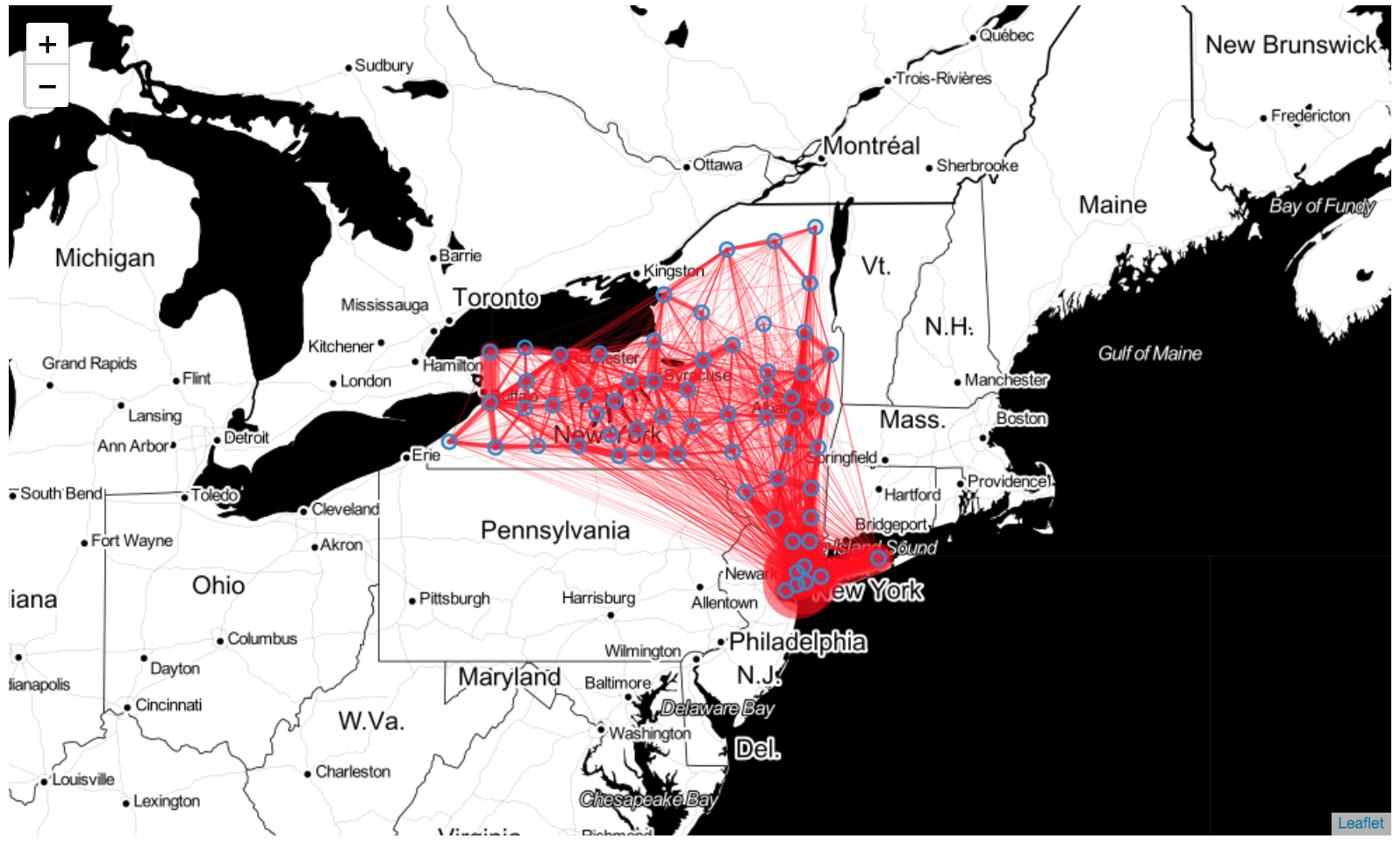
- plot_flows(map_f=None, min_flow=0, tiles='Stamen Toner', zoom=6, flow_color='red', opacity=0.5, flow_weight=5, flow_exp=0.5, style_function=<function <lambda>>, flow_popup=False, num_od_popup=5, tile_popup=True, radius_origin_point=5, color_origin_point='#3186cc', control_scale=True)
Plot the flows of a FlowDataFrame on a Folium map.
- Parameters
map_f (folium.Map, optional) – the folium.Map object where the flows will be plotted. If None, a new map will be created. The default is None.
min_flow (float, optional) – only flows larger than min_flow will be plotted. The default is 0.
tiles (str, optional) – folium’s tiles parameter. The default is Stamen Toner.
zoom (int, optional) – initial zoom of the map. The default is 6.
flow_color (str, optional) – the color of the flow edges. The default is red.
opacity (float, optional) – the opacity (alpha level) of the flow edges. The default is 0.5.
flow_weight (float, optional) – the weight factor used in the function to compute the thickness of the flow edges. The default is 5.
flow_exp (float, optional) – the weight exponent used in the function to compute the thickness of the flow edges. The default is 0.5.
style_function (lambda function, optional) – the GeoJson style function. The default is plot.flow_style_function.
flow_popup (boolean, optional) – if True, when clicking on a flow edge a popup window displaying information on the flow will appear. The default is False.
num_od_popup (int, optional) – number of origin-destination pairs to show in the popup window of each origin location. The default is 5.
tile_popup (boolean, optional) – if True, when clicking on a location marker a popup window displaying information on the flows departing from that location will appear. The default is True.
radius_origin_point (float, optional) – the size of the location markers. The default is 5.
color_origin_point (str, optional) – the color of the location markers. The default is ‘#3186cc’.
control_scale (boolean; optional) – if True, add scale information in the bottom left corner of the visualization. The default is True.
- Returns
the folium.Map object with the plotted flows.
- Return type
folium.Map
Examples
>>> import skmob
>>> import geopandas as gpd
>>> # load a spatial tessellation
>>> url_tess = skmob.utils.constants.NY_COUNTIES_2011
>>> tessellation = gpd.read_file(url_tess).rename(columns={'tile_id': 'tile_ID'})
>>> # load real flows into a FlowDataFrame
>>> # download the file with the real fluxes from: https://raw.githubusercontent.com/scikit-mobility/scikit-mobility/master/tutorial/data/NY_commuting_flows_2011.csv
>>> fdf = skmob.FlowDataFrame.from_file("NY_commuting_flows_2011.csv",
                                        tessellation=tessellation,
                                        tile_id='tile_ID',
                                        sep=",")
>>> print(fdf.head())
     flow origin destination
0  121606  36001       36001
1       5  36001       36005
2      29  36001       36007
3      11  36001       36017
4      30  36001       36019
>>> m = fdf.plot_flows(flow_color='red')
>>> m
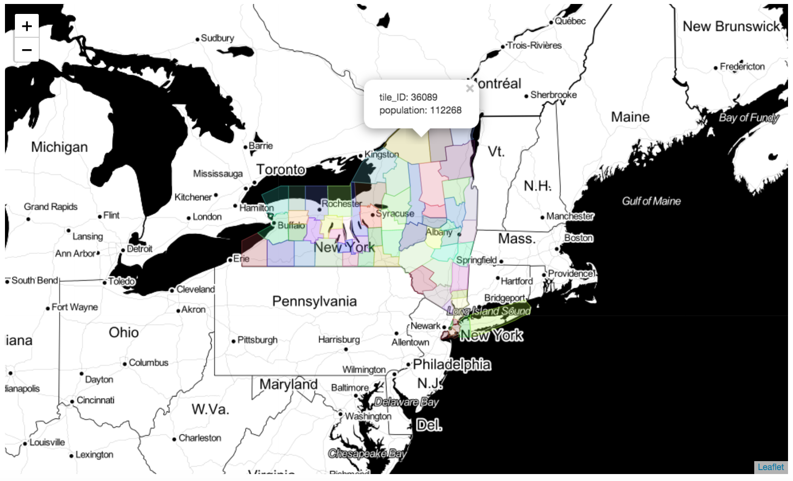
- plot_tessellation(map_f=None, maxitems=-1, style_func_args={}, popup_features=['tile_ID'], tiles='Stamen Toner', zoom=6, geom_col='geometry')
Plot the spatial tessellation on a Folium map.
- Parameters
map_f (folium.Map, optional) – the folium.Map object where the GeoDataFrame describing the spatial tessellation will be plotted. If None, a new map will be created. The default is None.
maxitems (int, optional) – maximum number of tiles to plot. If -1, all tiles will be plotted. The default is -1.
style_func_args (dict, optional) – a dictionary to pass the following style parameters (keys) to the GeoJson style function of the polygons: ‘weight’, ‘color’, ‘opacity’, ‘fillColor’, ‘fillOpacity’. The default is {}.
popup_features (list, optional) – when clicking on a tile polygon, a popup window displaying the information in the columns of gdf listed in popup_features will appear. The default is [constants.TILE_ID].
tiles (str, optional) – folium’s tiles parameter. The default is ‘Stamen Toner’.
zoom (int, optional) – the initial zoom of the map. The default is 6.
geom_col (str, optional) – the name of the geometry column of the GeoDataFrame representing the spatial tessellation. The default is ‘geometry’.
control_scale (boolean; optional) – if True, add scale information in the bottom left corner of the visualization. The default is True.
- Returns
the folium.Map object with the plotted GeoDataFrame.
- Return type
folium.Map
Examples
>>> import skmob
>>> import geopandas as gpd
>>> # load a spatial tessellation
>>> url_tess = skmob.utils.constants.NY_COUNTIES_2011
>>> tessellation = gpd.read_file(url_tess).rename(columns={'tile_id': 'tile_ID'})
>>> # load real flows into a FlowDataFrame
>>> # download the file with the real fluxes from: https://raw.githubusercontent.com/scikit-mobility/scikit-mobility/master/tutorial/data/NY_commuting_flows_2011.csv
>>> fdf = skmob.FlowDataFrame.from_file("NY_commuting_flows_2011.csv",
                                        tessellation=tessellation,
                                        tile_id='tile_ID',
                                        sep=",")
>>> m = fdf.plot_tessellation(popup_features=['tile_ID', 'population'])
>>> m
- settings_from(flowdataframe)
Copy the attributes from another FlowDataFrame.
- Parameters
flowdataframe (FlowDataFrame) – the FlowDataFrame from which to copy the attributes.
- class skmob.core.flowdataframe.FlowSeries(data=None, index=None, dtype: Dtype | None = None, name=None, copy: bool = False, fastpath: bool = False)